Modeling Synaptic Connections and Large Networks with G-3
Related Documentation:
Index of GENESIS 3 User Tutorials
Creating GENESIS 3 Simulations with Python
Creating a G-3 GUI with Python
Introduction
The tutorial Creating GENESIS 3 Simulations with Python describes the basics of creating simulation scripts in Python for single cell models. The tutorial begins with a demonstration script example that loads a simple two-compartment cell model 'simplecell' from a saved NDF file. It then continues to demonstrate ways to provide simulated experimental inputs to the cell, such as steady or pulsed injection currents, or random background synaptic excitation. Output of the simulation results is provided with the 'double_2_ascii' output object, which writes them to a file, similar to the GENESIS 2 'asc_file' command. This first part of the tutorial is necessary background for the present tutorial, which illustrates how to build simple circuits and large networks from a prototype cell. In particular, be sure to read the sections in the Introduction on 'Some background on the G-shell and the NDF file format' and 'Where are the example scripts and the graphical tools?'
Later, the python scripting tutorial continues to introduce other types of output objects such as 'live_output', to send the output to an accessible Python data structure (a list of lists) for plotting when the simulation is run, rather than to a file for later plotting. The tutorial concludes by converting the basic script into one that puts the non-gaphical parts of the simulation into a 'G-3 simulation object'. This provides the basis for the following tutorial Creating a G-3 GUI with Python. This tutorial adds a Control Panel and a graph, using a set of G-3 Python widgets that mimic the appearance and functionality of those used in GENESIS 2 with XODUS.
The present tutorial is based on non-graphical demonstration scripts that write results to a file, using external G-3 visualization tools for display. However, the information described in the previous paragraph for adding graphics to single cell models will be equally applicable for network models, and should later be consulted for further development of your network simulation scripts.
This preliminary version of the network modeling tutorial does not describe all of the options of some of the commands, some of which are untested or under development. For some very useful information from earlier GENESIS 2 tutorials, which will be later merged into the final version, it will be useful to take a brief look at Making synaptic connections and Creating large networks with GENESIS
The developer test scripts for the G-shell and SSPy components of G-3 provide a resource for obtaining the latest example scripts for network models implemented with G-shell or Python commands. These scripts often have tests for recently implemented features that have not yet been incorporated into the tutorials. Typically, new features are first implemented in the G-shell scripts, and then the Python bindings for the G-shell commands are tested with the Python scripts. After upgrading a G-3 installation (with 'neurospaces_upgrade', as described in the installation documents), examine some of the files in ~/neurospaces_project/gshell/source/snapshots/0/tests/scripts and ~/neurospaces_project/sspy/source/snapshots/0/tests/python.
Background
The GENESIS 2 tutorial Making synaptic connections uses the 'simplecell' model to illustrate the way that synaptic connections are created by connecting the soma compartment to a 'spikegen' object that delivers 'SPIKE' events to a synchan of another cell. In G-3, the process is very similar, but the soma, spikegen, and synchan are connected with 'messages' in GENESIS 2, whereas the connections in G-3 are somewhat different, as described in more detail in the following examples.
The following GENESIS 2 tutorial Creating large networks with GENESIS introduces the use of the powerful GENESIS commands createmap and planarconnect (or volumeconnect) to efficiently create large netorks of cells connected according to their locations on a rectangular grid. The cell used in the example simulation is a simple one-compartment cell model 'RScell' that has a firing pattern closer to that of typical cortical pyramidal cells, rather than the fast spiking 'simplecell' model that was used in the previous tutorials. Note that both of these cell models are available in the G-3 cells library, along with others that are described in Some NDF files of converted GENESIS 2 models.
This G-3 tutorial follows the organization of the two GENESIS 2 tutorials, beginning with a simple example of a cell-to-cell synaptic connection in the G-shell script two-cells.g3. However, instead of using the 'simplecell' model that was used in the previous G-3 and GENESIS 2 scripts, it uses the 'RScell' model from the outset.
The 'RScell' model
The 'RScell' is a very simple one-compartment model of a neocortical regular spiking pyramidal cell that, in addition to a fast sodium current and delayed rectifier potassium current, uses a Muscarinic potassium current (KM) in order to achieve spike frequency adaption. This model is based on a paper and NEURON simulation by Destexhe et al. (2001). These channels produce more realistic firing patterns than those used in the 'simplecell' model, which is more typical of a fast-spiking inhibitory interneuron. The simplicity of this cell model and the limited connectivity allows our example 'RSnet' network of 1024 neurons to run fairly quickly.
But, it is important to note that single-compartment models with only these three ionic conductances have limitations. Although the KM current may play a role in spike frequency adaption of cortical pyramidal cells, the behavior of these cells is largely determined by calcium currents and at least two varieties of calcium-activated potassium currents. You may explore the 'RScell' and explore its response to different types of inputs, as well as some more realistic cortical pyramidal cell models by modifiying some of the the previous G-3 single cell example scripts to use some of the other cells in the G-3 cells library. (See Some NDF files of converted GENESIS 2 models.)
Preliminary exercise:
Convert the simplecell_pulse.py script from Creating GENESIS 3 Simulations with Python to use the RScell, with the 0.05 sec current injection pulse of 1.5e-9 Ampere that is used in the RSnet model. Plot the results with the 'g3plot' tool. Alternatively, adapt the GUI used in Creating a G-3 GUI with Python to run the simulation from a Control Panel and view the plot of membrane potential.
The large network model used in the G-3 version of RSnet uses the G-3 implementation of createmap and the command createprojection, which is similar to the GENESIS 2 planarconnect command that was used in the original tutorial.
The 'RSnet' model
RSnet is a demonstration of a simple network, consisting of a square grid of simplified 'RScell' neocortical regular spiking pyramidal cells, each one coupled with excitory synaptic connections to its four nearest neighbors. A brief current injection pulse to the soma of a specified cell (typically in the center or lower left corner) starts a propagating wave of excitation. This simple connection pattern might model the connections due to local association fibers in a cortical network.
Like the original RSnet tutorial script, the Python example simulation RSnet.py given here was designed to be easily modified to allow you to use other cell models, implement other patterns of connectivity, or to augment it with a population of inhibitory interneurons and the several other types of connections in a cortical network.
The GENESIS 2 version has since been further extended to more biologically interesting networks with both excitatory and inhibitory connections, such as the Vogels and Abbott (2005) model GENESIS implementation with Hodgkin-Huxley dynamics. This was used as a benchmark for neural simulators in the review by Brette et al. (2007). This GENESIS implementation of a network benchmark would be a good project to implement in G-3, as an extension of RSnet.
Although the RSnet model is too simple to be of serious scientific interest without the extensions described above, it illustrates the same GENESIS objects and commands that are used in much more detailed cortical models. With no competing inhibition, the general behavior of the model can easily be understood, and the correct behavior recognized from an analysis of the output. or a visualization of the network acivity using the netview.py tool that is provided with G-3.
Making Synaptic Connections
Usually, we can treat an axon as a simple delay line for the delivery of spike events that last a single time step. Only if we are interested in understanding the details of axonal propagation would it be necessary to model the axon as a series of linked compartments.
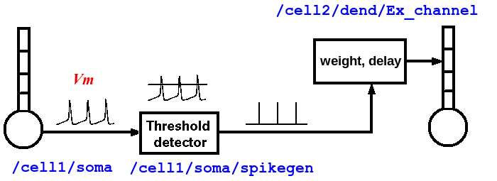
As shown in the diagram above, the properties of an axon are split between two types of GENESIS objects. Spiking class objects (e.g., a spikegen) create the spike events, when the membrane potential Vm crosses a threshold during an action potential. These send SPIKE events to a synchannel type element (synchan, and in the future, variations with learning), which contains fields for the propagation delays and synaptic weighting for each synaptic connection. As will seen in the examples below, this information is stored somewhat differently in G-3 than in GENESIS 2.
Typically, a spike is generated by the spikegen when the soma Vm exceeds the 'THRESHOLD' value of 0. In the RSnet examples below, the field 'REFRACTORY' has been set to 0.004 (4 msec) in order to prevent multiple spikes from being generated during the time that Vm is above threshold. Normally, REFRACTORY will be set to something greater than the maximum width of the action potential at threshold, and less than the minimum expected interspike interval. Note that the true absolute refractory period of a neuron is determined by the dynamics of the conductances that produce the action potentials. The REFRACTORY field of a spikegen can sometimes be useful for limiting the maximum rate of spike generation. However, it would only be used to set an absolute refractory period for firing when using highly simplified neuron models, or create artificial inputs that need to generate spikes with a specified minimum period.
two-cells.g3
The G-shell script, two-cells.g3 uses the RScell model with cell 1 having a steady injection current, and with soma action potentials generating spikegen events that are passed to cell 2 via a synaptic connection to the synchan Ex_channel. The connection between the cells uses a very large (30 msec) propagation delay in order to easily see the effect.
This script, and the other ones used in this tutorial may be obtained by downloading and saving the archive file network-scripting-examples.tar.gz, and extracting the files. If your browser does not permit this, you may save the files from the individual links given here. However, they will have a '.txt' extension in order to allow display as a text file.
The script begins with:
ndf_load_library rscell cells/RScell-nolib2.ndf
Note that instead of using the 'ndf_load' command, as in single cell simulation scripts, this uses the command 'ndf_load_library', which loads an ndf file into a namespace and reconstructs the model it describes within that namespace. This allows the model in the namespace to be used as a prototype for efficiently creating copies. 'ndf_load_library' should be contrasted with 'ndf_load', which simply reconstructs the model. For further information on G-3 namespaces, see the documentation on Namespaces in the Model-Container and the Neurospaces Description Format and the documentation for The NDF File Format.
In this example, the command creates the namespace '::rscell::' with a prototype cell having the elements /cell/soma, /cell/soma/Ex_channel, etc.
The excitatory synchan of the cell used to build the network will have the default parameters given in the NDF file. Typically the conductance density and the reversal potential will need to be set to a more appropriate value. The following lines set these values:
model_parameter_add ::rscell::/cell/soma/Ex_channel G_MAX 0.04330736624
model_parameter_add ::rscell::/cell/soma/Ex_channel Erev 0
Here the actual conductance in Siemens is G_MAX * soma_area, where soma_area can be calculated from the dimensions of the compartment (a sphere of diameter 105 micrometers, or cylinder of length and diameter of 105e-6 m) to be 3.463609149e-08 m^2.
In principle, the absolute value of 1.5e-9 S could be set directly. In RScell-nolib2.ndf, G_MAX is stored as a conductance density and scaled to the surface area by the model-container when it is fetched by a solver. Note that the model-container implements the scaling operation. A parameter instance would in principle be scaled, but should not be scaled when it is fetched by the solver. It should be defined in the NDF file with the 'FIXED' function.
An NDF example of 'fixing' a parameter at a chosen value is (from channels/nmda.ndf):
PARAMETERS
      PARAMETER ( Erev = 0.0 ),
      PARAMETER ( G_MAX = FIXED ( PARAMETER ( value = 6.870657376e-10),
PARAMETER ( scale = 1 ), ), ),
END PARAMETERS
However, it is not possible to attach functions (FIXED or other) to parameters from the gshell or sspy at present. For now, the conductance density should be calculated from the compartment dimensions and fixed value, then set with 'model_parameter_add'.
Next, a network element is created to be the root of the hierarchy of cells:
create network /two_cells
The next two commands create the two components '/two_cells/1' and '/two_cells/2' as references to '::rscell::/cell', with the same parameters, including the values of the synchan G_MAX and Erev that were set previously in the namespace prototype:
insert_alias ::rscell::/cell /two_cells/1
insert_alias ::rscell::/cell /two_cells/2
Here, '1' and '2' behave as copies of the prototype cell. Internally they are stored in a compact graph that reduces the memory footprint of the model. For more details on the representation of synaptic connections, see the section below 'Storage of connection information in G-3'.
To connect the two cells '1' and '2' together in a simple network, we need to create a projection element:
create projection /two_cells/projection
Note that this is not the same as the 'createprojection' command, which is described later below. A projection holds a group of connections between cells. In this example, there is only one connection: a synaptic connection between the spike generator in the soma of cell 1, and the excitatory synchan in cell 2. The connection is created with the statements:
model_parameter_add /two_cells/projection SOURCE /two_cells
model_parameter_add /two_cells/projection TARGET /two_cells
This means that source and target of the connection (or possible multiple connections) will involve cells in the '/two_cells' population. To make a connection that originates in cell 1, we need to provide a 'connection symbol' that can be used to refer to this connection and to hold the parameters of the connection:
create connection_symbol /two_cells/projection/1
The '1' is an arbitrary chosen name of the connection, and is not referencing cell 1. A second connection could be called '2' or even 'second_connection' or whatever the user chooses.
Then, connection '1' is given the parameters needed to have a presynaptic event come from the spike generator in the soma of cell 1, and a postsynaptic event to occur at a synapse formed with the Ex_channel in cell 2:
model_parameter_add /two_cells/projection/1 PRE 1/soma/spike
model_parameter_add /two_cells/projection/1 POST 2/soma/Ex_channel/synapse
model_parameter_add /two_cells/projection/1 WEIGHT 2.0
model_parameter_add /two_cells/projection/1 DELAY 0.03
Note that, unlike GENESIS 2, in which the synaptic weight and propagation delay are stored in the synapse of the target neuron, here they are stored in the connection symbol for the connection '1'.
Next, add an injection current to the cell 1 soma, and provide outputs of relevant parameters:
inputclass_add perfectclamp current_injection_protocol name current_injection command 1e-9
input_add current_injection_protocol /two_cells/1/soma INJECT
output_add /two_cells/1/soma Vm
output_add /two_cells/2/soma Vm
output_add /two_cells/2/soma/Ex_channel Gsyn
output_add /two_cells/2/soma/Ex_channel Isyn
These are commands are similar to the ones used in single cell simulations for input and output. Note the use of the alias to allow references to individual cells. As no output file name was specified, the output will go to the default file '/tmp/output'.
Finally we need to set up the solvers to be used. As with single cell models, Heccer is used to perform the computations for the cells. However the Discrete Event Solver (DES) is needed for the synaptic connections in the network. First, some commands are used to configure the solvers:
heccer_set_config disassem_simple
des_set_config disassem_simple
In thse statements, 'disassem_simple' is the name of a configuration that is used for development. In the future, the default configuration may be used here, and the 'set_config' commands may be eliminated.
The 'set_verbose' command can be used to control the amount of output is generated when the model is set up and run:
set_verbose debug
This line will normally be commented out to prevent a flood of detail, or set to a lower verbosity level. The use of this command is described in the G-shell documentation The GENESIS 3 Shell Software Component.
Then, we assign the Heccer solver to the cells, and DES to the projection:
solverset /two_cells/1 heccer
solverset /two_cells/2 heccer
solverset /two_cells/projection des
Finally, the model is run, as usual:
run /two_cells 0.2
The script can be run with the command:
$ genesis-g3 two-cells.g3
At this point, you may enter gshell commands to explore the network, for example:
genesis > list_elements /two_cells
---
- /two_cells/1
- /two_cells/2
- /two_cells/projection
 genesis > list_elements /two_cells/2/soma
 ---
- /two_cells/2/soma/Na_pyr_dp
- /two_cells/2/soma/Kdr_pyr_dp
- /two_cells/2/soma/KM_pyr_dp
- /two_cells/2/soma/Ex_channel
- /two_cells/2/soma/spike
The network can be explored in more detail by invoking the Studio from the G-shell using explore command:
genesis > explore
To explore the structure of the constructed model, choose the 'Explorer' menu button in the window that pops up. You can then browse the model in the left panel of the window that pops up by double clicking. In the title of each window that is openend, you see the full path name of the model element you are inspecting. Use the 'Quit' menu button to close all the windows and return control to the command line shell.
For some more information on the use of the Studio to explore connections. see the Notes on using the Neurospaces Studio.
When you are finished, give the command:
genesis > quit
At this point, you will find a file in /tmp/output which you may examine with the 'g3plot' tool:
$ g3plot /tmp/output
The plot should look like this:
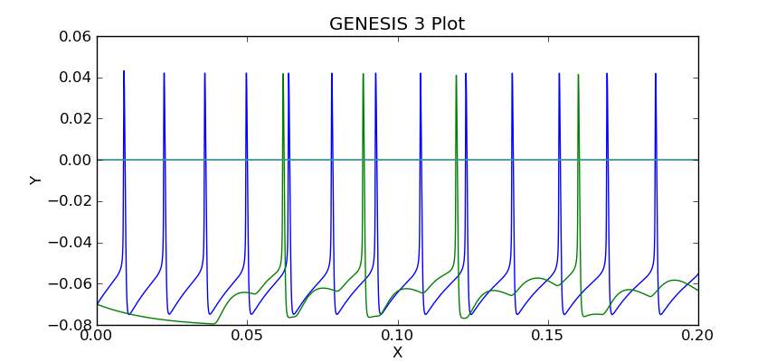
Note the delay before cell 2 responds to the spikes generated by cell 1. The magnitudes of the synaptic conductance and current are much smaller than the membrane potentials, so one would use the "zoom" tool to inspect them, unless they were plotted separately, or saved to a different file.
The next example illustrates the "memory efficient" method of constructing large networks. But first, it is time for some more explanation of the way that synaptic connections are treated in G-3.
Storage of connection information in G-3
There are two ways to store connection information in the G-3 Model Container:
1. The 'two-cells.g3' script illustrates the use of a 'connection_symbol' to hold the information for each synaptic connection. This type of "flexible connection" can be useful when a model requires very specific individual cell-to-cell connections that cannot be generated from the algorithms that are available with the 'createprojection' command. It also makes it possible to set the connection parameters for any connection individually. However, when storing the individual connections in a large, highly connected network model, this method uses a great deal of memory, and is not very efficient.
2. The 'rsnet-2x2-createprojection' script illustrates the second way, using the 'createprojection' command. It is assumed that the cells lie on one or more two-dimensional grids of equally spaced points, created with the 'createmap' command and connected according to options specified with the 'createprojection' command. These "memory-efficient" connections use a fixed set of parameters, currently pre- and post-synaptic target serial identifiers and delay and weight of the connection. Memory efficient connections don't have a user-chosen label, as is done with flexible connections.
For more details on the representation of synaptic connections, see the Technical Notes on Connections. The document Model of a Connection describes how synaptic connection information is stored in the NDF format.
The rsnet-2x2-createprojection script
The G-shell was not designed to be a full programming language with loops, conditionals, nor other features found in languages such as Perl or Python. When creating simulations that involve many cells, either a 'wildcard' notation is needed or a mechanism to interate over the cells in the network. Therefore the script 'rsnet-2x2-createprojection' is written in Perl in order to provide an interface to the gshell functions used to create and simulate the network.
As the Python example to be given later provides a more user-friendly way to do the same thing, the following description will concentrate only on the commands that illustrate the 'memory efficient' method of creating a network, and the notation that will be used any scripting language that implements these commands. Normally, only developers will use Perl for scripting test cases.
The script rsnet-2x2-createprojection begins with a header identifying it to be executed as a Perl script, with display of warnings:
#!/usr/bin/perl -w
and continues with some definitions needed to find the needed paths and modules. Then it defines the values of NX, NY, SEP_X, SEP_Y, SEP_Z, as well as the synaptic weights and delays of the connections.
As in the previous example, the script uses:
ndf_load_library('rscell', 'cells/RScell-nolib2.ndf');
followed by 'model_parameter_add' commands to change some properties of the excitatory synchan 'Ex_channel' in the prototype cell. Then the network object is creaed with:
create('network', '/RSNet');
At this point, the namespace '::rscell::/' has been created with the cell prototype. However, the work of creating the cells is performed, not by creating an alias for each cell, but with a more efficient algorithm that creates a representation of the prototype cell at points on a rectangular grid. The are NX points along the x-axis, with a spacing SEP_X, and NY points along the y-axis, with a spacing SEP_Y. The cells are numbered from 0 to NX*NY - 1. In this scaled down test example, NX and NY are set to 2, but a network of any size can be created by changing these variables. The 'createmap' command takes these arguments:
createmap('::rscell::/cell', '/RSNet/population', $NX, $NY, $SEP_X, $SEP_Y);
Then the 'createprojection' command is used, not only to create the projection used for connections within this population of cells, but also the connections within the projection. The createprojection command has many parameters to cover various algorithms for creating connections between cells. The ones needed for variations of the RSnet model are given in the Perl code:
createprojection (
   {
    root => '/RSNet',
    projection => {
        name => '/RSNet/projection',
                  },
    source => {
        context => '/RSNet/population',
        include => {
                   type => 'box', # type => 'all' removes need for line below
                   coordinates => [ '-1', '-1', '-1', '1', '1', '1', ],
                  },
              },
    target => {
        context => '/RSNet/population',
        include => {
                   type => 'ellipse',
                   coordinates => [ 0, 0, 0, $SEP_X * 1.2, $SEP_Y * 1.2, $SEP_Z * 0.5, ],
                   },
        exclude => {
                   type => 'box',
                   coordinates => [ -$SEP_X * 0.5, -$SEP_Y * 0.5, -$SEP_Z * 0.5,
                     $SEP_X * 0.5, $SEP_Y * 0.5, $SEP_Z * 0.5, ],
                  },
              },
    synapse => {
        pre => 'spike',
        post => 'Ex_channel',
        weight => {
                   value => $syn_weight,
                  },
        delay => {
                  value => $prop_delay,
                 },
               },
    probability => '1.0',
    random_seed => '1212.0',
   },
);
The meaning of the keywords 'include' and 'exclude' in the context of this model can best be seen in this figure:
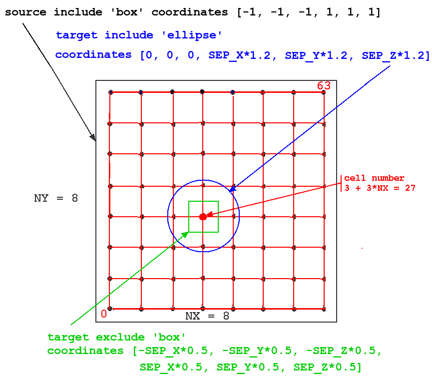
The figure illustrates how these options would be applied to a network of 64 cells with NX = NY = 8. The particular source cell for the connections shown (one of all in the source 'include' region, i.e. all of cells) is number 3 + 3*NX = 27.
In this simulation, we want to connect each source spike generator to the excitatory synchans on the four nearest neighbors. To do this, we define the source 'include' region to be a rectangle (box) with a very large range (-1 to +1 meters in each direction!), so that every cell in the network will be treated as a source.
We want the target for the connections, relative to the source, to be an ellipse (or circle) that is large enough to include the four neighbors. It is generally a good idea to set the target ellipse axes or box size somewhat higher than the cell spacing, to be sure that the cells are included. Although this isn't a problem with our single-compartment cell, it can be an issue if the target synapses are located in a distal dendrite compartment that is displaced by some amount from the cell origin. In this case it is an ellipsoid centered on (0,0,0), and having principal axes of length equal to 1,2 times the cell separation.
We also want to define a target 'exclude' region that excludes the source cell, so that it doesn't connect to itself. This is done by defining the region to be a box centered on the source, with sides equal to the half cell separation in each direction.
The probability of a connection is set to 1.0, so all connections will be made that fit this prescription. A random number seed is set for making probabilistic connections, but it is not used in this case.
To connect to nearest neighbors and the 4 diagonal neighbors, we would use a box for the target include that is slighly larger than the desired region, e.g.:
include => {
           type => 'box',
           coordinates => [ -$SEP_X*1.01, -$SEP_Y*1.01, -$SEP_Z*1.01,
             $SEP_X * 1.2, $SEP_Y * 1.2, $SEP_Z * 0.5, ],
           },
For all-to-all connections with a 10% probability, set both the source and target include region to have a range much greater than the size of the network, and 'probability' to 0.1.
The remainder of the script sets up a current injection to the soma of cell 3, refered to as '/RSNet/population/3', and uses a loop to provide output from each cell.
Likewise a loop is used to set Heccer as the solver for each cell, and a single 'solverset' command is used to set DES as the solver for the projection.
The script ends with the commented-out statement:
# explore();
If the '#' is removed, the script will invoke the Studio, so that you may explore the model before quitting the simulation.
The rsnet-2x2-createprojection script may be run with the command:
$ rsnet-2x2-createprojection
Then, the file in /tmp/output can be plotted with the 'g3plot' tool:
$ g3plot /tmp/output
The plot should look like this:
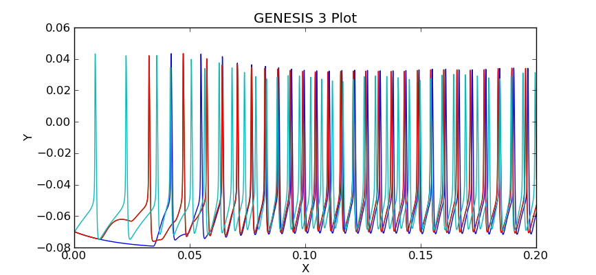
Can you see the activity in cell 3 propagate, causing cells 2 and 1 to fire, which then cause cell 0 to fire?
rsnet-32x32-createprojection.pl
The final G-shell/Perl example rsnet-32x32-createprojection.pl extends this model to the full 32x32 network, with some additions and changes in addition to setting NX and NY to 32, rather than 2.
- A variable for the simulation time $tmax has been added, so that the the simulation may be run with run('/RSNet', $tmax);
- The small 20e-06 time step (20 microsec) is far more resolution than is needed for the analysis of the network firing. An output step of 0.2 msec should be enough to represent action potentials, so we use the statement output_time_step(0.0002); to set the output interval. This significantly reduces the size of the output file.
- In order to generate an output suitable for the 'netview.py' network viewer, each line of the file should consist of just the Vm values of the 1024 cells at that output step, without the simulation time. This is done with the statement output_emit_time(0);.
Although it was not done in this script, you may specify a different output file than the default '/tmp/output' with a statement such as:
output_filename('rsnet-32x32-Vm.txt');
As with rsnet-2x2-createprojection.pl, you may run the script on the command line by typing the name, and explore the model if the final line that invokes 'explore' is uncommented.
You may determine the number of lines in the output file with the command:
$ wc /tmp/output
  2500  2560000 27868545 /tmp/output
A significant difference between G-shell and Python outputs is that the G-shell version does not produce an output for time and step 0, but begins with the first step.
For 1024 cells and this small (20 microsec) time step, the simulation can take over a minute to complete. In principle, the considerable setup time for storing the connection information could be avoided for subsequent runs that use the same connections, but different cell model parameters. Often, much of the "tuning" of a network model involves modifying the synchan model conductance G_MAX or its time constants. This feature has not yet been implemented in the G-shell simulation examples.
The behavior of the 2x2 network can be understood by plotting the membrane potenial of the four cells with 'g3plot'. In order to visualize the behavior of a large network, one needs other tools. The G-3 application 'netview.py" was developed as viewer simililar to the GENESIS 2 'xview' widget, and will be installed with 'g3plot' and the other tools in the G3Plot package. A development version of 'netview.py' has been included in the archive network-scripting-examples.tar.gz with the example scripts.
To use the viewer, give the command:
$ netview.py /tmp/output
and look at the Help/Usage menu for detailed instructions. This explains the optional header line that a data file may have with necessary network parameter information.
click "New Data". As this file has no header, a dialog box appears asking for the following parameters (and providing default values):
Number of entries (number of lines in file): 1250
Start time: 0.0002
  (normally it will be 0.0, but the first time is step 1).
Output time step: 0.0002
Number of cells on x-axis (NX): 32
Number of cells on y-axis (NY): 32
Note, that in order to enter the values, it is necessary to hit "Enter" in a text field for the value to register. This "feature" (present in GENESIS 2 XODUS also) could be changed with more sophisticated validation procedures for entries in the "XDialog" widget. (A nice project for someone with wxPython programming skills.)
After changing any of the default values that need to be changed, clik "OK". The display area will turn black, and a status message will appear at the bottom "Data has been loaded - click PLay"
Click "Play" and watch the activation spread out from the center. You may now use the sliders to replay during a particular time period, or Single Step to advance a frame. The Forward/Back toggle can move backwards and the Normal/Fast toggle can be used to play every 10th frame.
This G-shell implementation of RSnet will be the basis of Python examples to follow. However, it gives a steady injection to the center cell, rather than a single 0.05 sec pulse. This will be possible with future G-shell bindings to the pulsegen object, as was done in Python. However, this may be done more conveniently in a Python script such as the single cell example simplecell_pulse_sim.py. This will be the basis of the final example script 'RSnet.py'.
Implementing RSnet in Python
The example script RSnet.py is still under construction while the Python bindings are being implemented for the commands used in rsnet-32x32-createprojection.pl.
In the interim, check often for new Python network test scripts in your directory:
~/neurospaces_project/sspy/source/snapshots/0/tests/python
after performing 'neurospaces_upgrade' (or to just upgrade the SSPy module, 'neurospaces_upgrade --regex sspy').
Suggested Exercises
Of course, the first exercise should be to implement the unfinished 'RSnet.py' model as described above, using the logic of the G-shell/Perl version, the syntax of working Python test scripts, and the framework of simplecell_pulse_sim.py.
There many variations of the RSnet model that you can try in either the Python or G-shell/Perl examples. You can experiment with the effect of different propagation delays, weights or patterns of connections. For longer range connections that the nearest neighbor connnectivity used here, explore some of the createprojection options for random connectivity, or delays based on separation and conduction velocity. (These have not been well tested at the time this tutorial was written.)
However, as suggested earlier, the first step in creating a realistic cortical model is to add a population of inhibitory neurons, as was done in the well-documented GENESIS 2 implementation of the Vogels and Abbott (2005) model.
A typical simple cortical model contains a population of regular spiking pyramidal or stellate cells (e.g. the 'RScell' or a more realistic cell from the models library). These make excitatory connections not only with each other, but with a smaller population of inhibitory fast spiking basket cells (e.g. a 'simplecell'). These can make inhibitory connections with each other, or with the pyramidal cells. Thus, there will be two populations and four different projections in this model to represent the different source and target combinations.
There are typically about 25% as many inhibitory cells as excitatory cells in such a network. Try adding the inhibitory cell population as a 16 x 16 grid of cells that have twice the separation as the RScells. If the 'origin' option for 'createmap' has been implemented at this time, the origin of the cells on this grid should be displaced so that they fall in between the excitatory cells.
For a given choice of connectivity (short range or long range), there are many experiments that you can do to achieve a balance of excitation and inhibition in such a network.
Have fun!
References
Destexhe, A., Rudolph, M., Fellous, J. M. and Sejnowski, T. J. (2001) Fluctuating synaptic conductances recreate in-vivo-like activity in neocortical neurons. Neuroscience 107: 13-24.
Vogels TP, Abbott LF. (2005) Signal propagation and logic gating in networks of integrate-and-fire neurons. J. Neurosci. 25: 10786-10795.
Brette et al., (2007)
Brette R, Rudolph M, Carnevale T, Hines M, Beeman D, Bower JM, Diesmann M, Morrison A, Goodman PH, Harris Jr FC, Zirpe M, Natschlager T, Pecevski D, Ermentrout B, Djurfeldt M, Lansner A, Rochel O, Vieville T, Muller E, Davison AP, El Boustani S, and Destexhe A (2007). Simulation of networks of spiking neurons: a review of tools and strategies. J. Comput. Neurosci. 23: 349-398.